Thermofluids · NP-002
Thermodynamics Lab Series
Five practicals on what it costs to move heat: a Peltier element, gas expansion, two vapour-compression rigs and a four-stroke engine. Recorded, reduced, uncertainty-checked, and honest about the two that went wrong.
Measured ET 102 heat-pump cycle · R134a log p–h · dome from tabulated data, approximate near the critical point
00 · Overview
Five rigs, one thread: the cost of moving heat
Every rig in this unit does the same basic thing: it moves heat in a direction it wouldn’t go on its own, and something has to pay for that in work. Three of the experiments are heat pumps judged on coefficient of performance: one with electrons crossing a semiconductor junction, two with a refrigerant changing phase. One isolates the gas property that governs compression, and the last applies it to a spark-ignition engine.
Every measured number comes from data we recorded, and each measured experiment carries its own uncertainty budget, with instrument resolution treated as a rectangular distribution. Because none of the rigs came with calibration data, assumed accuracies are marked as assumptions.
3 of 5
Experiments that agreed well with theory (one is analytical)
82%
Of Carnot on the refrigerant side (ET 102)
3.7%
Gap between two independent resistance routes
±0.003
Resolution limit on κ, against a 1.39 scatter
01 · GUNT ET 120
Peltier cooling: one curve turns over, one keeps climbing
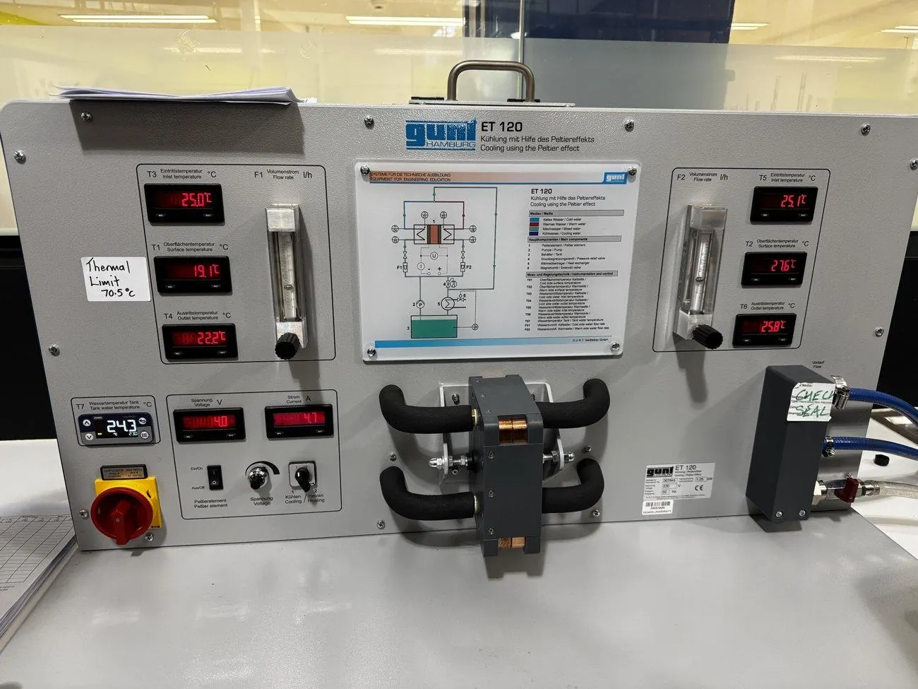
We stepped a Peltier element from 2 to 20 V and measured cooling capacity and heat output from energy balances on its two water circuits. Cooling peaks at a 70.7 W plateau between 14 and 17 V, then falls; the hot side climbs to 366 W. At the top of the range it dumps about six times the heat it removes.
The theory predicts exactly that shape: the Peltier term is linear in current, Joule heating is quadratic. The best check was independent: theory says Q̇h − Q̇c = I²R, so fitting the measured difference gave the element resistance as 1.061 Ω, against 1.022 Ω from a straight electrical regression.
COP fell from 4.11 to 0.15 and crossed 1.0 near 6 V. I flagged the 4.11 as unreliable: at 2 V the cold-side water changed by only 1.7 K on 4.8 W of input, the hot side by just 0.1 K (41% uncertainty), and the energy balance closed at only 19%.
02 · GUNT WL 103
Heat capacity ratio: diagnosing what went wrong
This one mostly didn’t work, and working out exactly why became part of the result.
The method compresses air into a tank, lets it cool back to ambient, then snaps a valve open for a near-adiabatic expansion. Only one of six determinations survived: κ = 1.304 ± 0.003, 6.9% below the textbook 1.40.
Four of the other five are physically impossible, and the fifth (1.09) used the wrong reference pressure. The recorded pressures show why. The tank wasn’t fully vented between runs (the starting pressure crept from 1.015 to 1.081 bar), and the valve was closed too early, so the expansion never reached atmospheric. For the two-tank method, we hadn’t recorded the pressure right after expansion at all.
Instrument resolution only accounts for ±0.003 in κ, while the three to-atmosphere runs scatter across 1.39, about 460 times larger. That’s as clear as evidence gets that the problem was procedure, not equipment.
I also ran the incomplete two-tank data backwards: assuming κ = 1.40, all three runs imply a post-expansion pressure between 0.94 and 0.96 bar. They’re consistent with each other, which suggests the data is incomplete rather than corrupt.
03 · GUNT ET 101
Simple refrigeration: when resolution dominates
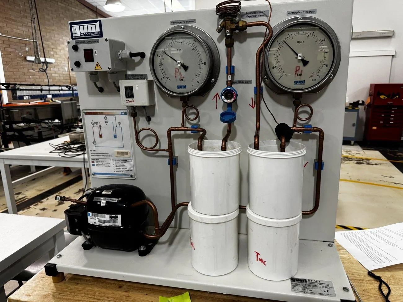
An R134a circuit with its evaporator and condenser coils sitting in buckets of water. Between 4 and 12 minutes the cold tank gave a refrigeration capacity of 17 ± 7 W (k = 2) and the condenser rejected 65.3 W.
The rig’s manometers read from −1 bar, which can only mean gauge pressure, so I converted to absolute before reading the chart. Mean pressures of 2.35 and 14.36 bar absolute give saturation temperatures of −6 and 53 °C.
The two mass-flow estimates disagreed by a factor of 2.8. The likely main cause is ambient heat leaking into the uninsulated cold tank. At roughly 10 W it’s comparable to the cooling itself, and allowing for it closes part of the gap. Water temperatures were also only read to the nearest degree. Insulated tanks and a 0.1 °C display would fix the biggest systematic and random errors together.
04 · GUNT ET 102
Heat pump: 82% of Carnot, 25% overall
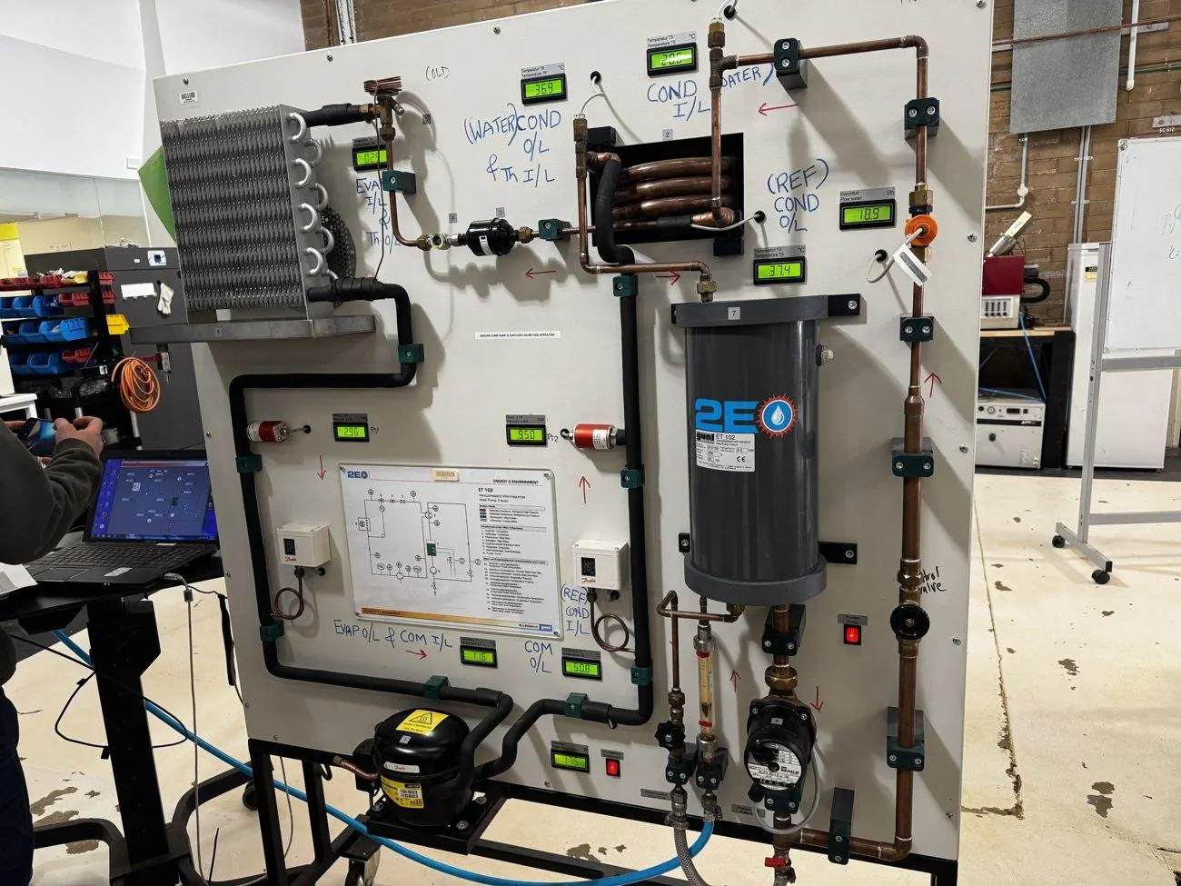
175 W into the compressor put 389.5 W into the hot-water loop, a measured COP of 2.23 ± 0.11. Three numbers describe the same machine, and the gaps between them say where the energy goes.
- Carnot limit2.9 °C → 38.1 °C8.84
- Refrigerant side(h₂ − h₃) / (h₂ − h₁)7.21
- MeasuredQ̇ water / P electrical2.23
−18 ptsCarnot → refrigerant side, in points of the Carnot limit (100% → 81.6%). The cycle’s own irreversibility: mostly throttling across the expansion valve, plus heat rejected above the condensing temperature and pressure drops in the pipework.
−56 ptsRefrigerant side → measured (81.6% → 25.2%). This gap is machinery, not thermodynamics. Only 54 W of the 175 W drawn reaches the refrigerant; the rest is motor, friction and valve losses.
From the measured refrigerant states the cycle gives COPHP = 7.21 and COPR = 6.21, differing by exactly 1, as they must. Matching the condenser duty to the water side gives a refrigerant flow of 7.88 kg/h and 54.1 W of compression work: only 31% of the electrical input.
I checked the pressure scale independently: R134a saturates at about 38.1 °C at 9.66 bar absolute, and the measured condensation temperature was 37.8 °C. If the readings were gauge, saturation would sit near 42 °C. That’s a 4 K mismatch, and an obvious one.
The same operating point was logged three ways (data sheet, software and panel) and gave COPs from 2.04 to 2.23. I reported the spread instead of quietly picking one.
05 · Cutaway engine
Four-stroke engine: geometry and the Otto limit
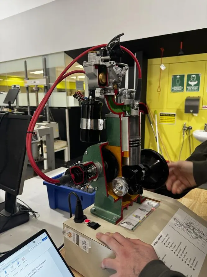
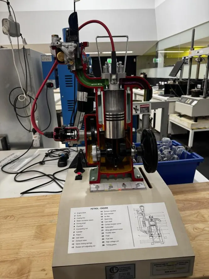
On a sectioned single-cylinder engine I identified the major components and followed the four strokes through two crank revolutions: one power stroke per two turns, with the camshaft geared at half speed.
For the given geometry (180 mm bore, 250 mm stroke, 50 mm clearance) the swept volume is 6,362 cm³, the clearance volume 1,272 cm³ and the compression ratio exactly 6.00, giving an ideal Otto efficiency of 51.2%.
The manual gave the clearance as “a volume of 50 mm”. That’s a length, and its figure dimensions it as the gap above the piston at TDC, so I treated it that way. Read as 50 cm³, the compression ratio would be 128, far beyond any real engine.
Interactive · Experiment 5 meets Experiment 2
How much does κ matter?
Ideal Otto efficiency is η = 1 − r1−γ. The only fluid property in it is γ, the same κ I tried to measure in Experiment 2. Move the compression ratio and compare the textbook 1.40 with my one valid measurement, 1.304.
- Efficiency, γ = 1.40
- 51.2%
- Efficiency, γ = 1.304
- 42.0%
- Difference
- 9.2 pts
A 7% drop in κ costs about 9 percentage points of ideal efficiency at r = 6. A real engine of this type would probably manage 25–30% brake thermal efficiency, roughly half the ideal figure. Combustion time, heat loss, friction and pumping all take their share.
06 · Summary
Headline results
| Exp. | Quantity | Measured | Expected | Note |
|---|---|---|---|---|
| 1 | Peak cooling capacity | 70.7 ± 3.5 W | — | Plateau across 14–17 V |
| 1 | Element resistance (thermal route) | 1.061 Ω | 1.022 Ω (electrical) | Two independent routes agree |
| 2 | Adiabatic exponent κ, set A1 | 1.304 ± 0.003 | 1.400 | −6.9% |
| 3 | Refrigeration capacity | 17 ± 7 W (k = 2) | — | 1 °C display resolution dominates |
| 4 | Heat pump COP, measured | 2.23 ± 0.11 | 8.84 (Carnot) | 25% of the limit |
| 4 | Heat pump COP, refrigerant side | 7.21 | 8.84 (Carnot) | 82% of the limit |
| 5 | Compression ratio / ideal Otto efficiency | 6.00 / 51.2% | — | Exact by construction |
07 · Lessons
What I took away
Two routes beat one
The most useful checks compared two independent routes to the same number: thermal vs electrical resistance, refrigerant vs water-side mass flow, measured vs saturation temperature. A measurement on its own is hard to trust.
Resolution isn’t trivial
Display resolution decided two of five results. Reading water temperature to the nearest degree capped one result at two significant figures. In another, a 0.1 °C display against a 0.1 K hot-side rise left the low-voltage point unmeasurable.
Every measured COP is a lower bound
Uninsulated rigs on an open bench lose heat everywhere (a 25% energy-balance shortfall, ambient gain, pipework losses), and every one of those biases measured performance downwards.